Data Point (a.k.a example or observation)
Data Set
Outliers
Construct
Operational Definition
The operational definition of a construct is the unit of measurement we are using for the construct. Once we operationally define something, it is no longer a construct. If we define area in sft, then this would be operationally defined. E.g.; Minutes is already operationally defined; there is no ambiguity in what we are measuring.
Treatment
Observational Study
Treatment Group
Control Group
Independent Variable (a.k.a feature, predictor variable, input variable in machine learning. In a tabular data, every column may correspond to a feature.)
Dependent Variable (a.k.a output variable, target variable, outcome variable, predicted variable in machine learning.)
Confounding Variable (a.k.a factor)
Control Variable
Normalization or Min-Max Scaling or Scaling Normalization
In this technique the values are transformed to be in the range of 0-1 or -1 to 1.
This way it helps to bring multiple features to the same scale so that one feature does not influence greater or lesser than the other while model building.
The formula for getting 0-1;
x_new = (x - x_min)/(x_max - x_min)
Normalization is ideally applied after removing the outliers.
Standardization or Z-Score Normalization
In this the values are transformed to have a mean value of 0 and its standard deviation is 1
The formula is;
x_new = (x - x_mean)/x_std - where std is the standard deviation`
x_new is also called the z-score. Any normal distribution can be converted to Standard normal distribution by plotting the computed z-scores. In a Standard normal distribution the mean is 0 and standard deviation is 1.
Z-scores are not affected by outliers and there is no upper or lower bound like in Normalization.
Central Limit Theorem
Central Limit Theorem states that: If you randomly pick up samples of a population and calculate the arithmetic mean of these individual samples, then, if you plot the arithmetic mean of samples, it will closely approximate a normal distribution if the number of samples taken are very large - close to infinity. This is true even if the population itself is not a normal distribution. And if you now compute the mean of the means of various samples, it closely represents the population mean. This mean of means is called the 'point estimate' - a type of statistic
Standard Error
Standard Error is nothing but the standard deviation of various sample statistics (check the central limit theorem above) - such as the mean or median. If the standard error is small then it means the statistic closely represents the population parameter.
Variance
Coefficient of Variation (a.k.a relative standard deviation)
The coefficient of variation (CV) is defined as the ratio of the standard deviation to the mean
- StandardDeviation/mean - gives this value
To compare apples to apples, you calculate the CV of two datasets and then their variability. E.g, Compare variability of SAT scores of students in Math and English
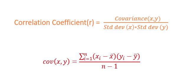
Covariance and Correlation
Confidence Level
It is the level of confidence expressed in percentage, that basically tells what percentage of times you expect to reproduce an estimate of the population parameter between the upper and lower bounds of the confidence interval.
For e.g., you are correct 95% of the times, when you say that the mean age of students in 11th grade in any school is between 15 and 19
If you increase the confidence level, you will be forced to increase the confidence interval. So for e.g., you are correct 100% of the time when you increase the mean age range between 1 and 130
Confidence Interval or Error Bars
Discreet Variable
Continuous Variable
Frequency Distribution
The count of the number of occurrence of each distinct value of a variable. Usually applied to categorical variables.
Null Hypothesis
the Null hypothesis represents the status quo or the existing belief, while the alternative hypothesis represents the researcher's claim or the new idea that they are testing.
Typically, the null hypothesis represents the absence of an effect or the lack of a difference between groups, while the alternative hypothesis represents the presence of an effect or a difference between groups.
Examples:
- A researcher might hypothesize that a new drug is more effective at treating a particular condition than a placebo. The null hypothesis would be that the drug is no more effective than the placebo. The researcher would then conduct a clinical trial, randomly assigning patients to receive either the drug or the placebo, and measure the outcomes. The data collected would be analyzed using null hypothesis testing to determine whether there is enough evidence to reject the null hypothesis and conclude that the drug is indeed more effective than the placebo.
- A company might use null hypothesis testing to determine whether a new manufacturing process produces products that are more consistent than the old process. The null hypothesis would be that the new process does not produce more consistent products than the old process. The company would collect data on product consistency and analyze it using null hypothesis testing to determine whether there is enough evidence to reject the null hypothesis and conclude that the new process does indeed produce more consistent products.
A complete example with calculations:
Suppose we are testing a new fertilizer that is claimed to increase crop yields. We randomly select 20 fields and apply the fertilizer to half of them, while the other half receives no treatment. After the harvest, we measure the yield of each field in bushels per acre.
Our null hypothesis is that the mean yield of the fields that received the fertilizer is the same as the mean yield of the fields that received no treatment. Our alternative hypothesis is that the mean yield of the fields that received the fertilizer is greater than the mean yield of the fields that received no treatment.
We can express these hypotheses mathematically as follows:
H0: µ1 = µ2
Ha: µ1 > µ2
where H0 is the null hypothesis, Ha is the alternative hypothesis, µ1 is the mean yield of the fields that received the fertilizer, and µ2 is the mean yield of the fields that received no treatment.
To test these hypotheses, we can calculate the sample means and standard deviations of the two groups, and use a t-test to determine whether the difference in means is statistically significant. The t-test statistic can be calculated as follows:
t = (x1 - x2) / (s / sqrt(n))
where x1 and x2 are the sample means of the two groups, s is the pooled standard deviation of the two groups, n is the sample size, and the denominator is the standard error of the difference in means.
Suppose that our sample means and standard deviations are as follows:
- x1 = 225 bushels per acre (mean yield of fields with fertilizer)
- x2 = 200 bushels per acre (mean yield of fields without fertilizer)
- s1 = 20 bushels per acre (standard deviation of yields with fertilizer)
- s2 = 25 bushels per acre (standard deviation of yields without fertilizer)
- n = 10 (sample size for each group)
Using these values, we can calculate the pooled standard deviation as follows:
s = sqrt(((n1 - 1) * s1^2 + (n2 - 1) * s2^2) / (n1 + n2 - 2))

  = sqrt(((9 * 20^2) + (9 * 25^2)) / 18)

  = 22.45 bushels per acre
Using the t-test formula, we can calculate the t-statistic as follows:
t = (225 - 200) / (22.45 / sqrt(10))

  = 3.06
We can then use a t-table or statistical software to determine the p-value associated with this t-statistic. Assuming a significance level of 0.05, we find that the p-value is less than 0.05, which means that we can reject the null hypothesis and conclude that the fertilizer does indeed increase crop yields.
t-table values for degrees of freedom (df) ranging from 1 to 30
- at significance levels of 0.10, 0.05, and 0.01:
| df | 0.10 | 0.05 | 0.01 |
|---|---|---|---|
| 1 | 1.32 | 1.72 | 6.31 |
| 2 | 1.08 | 1.60 | 2.92 |
| 3 | 0.88 | 1.42 | 2.35 |
| 4 | 0.76 | 1.20 | 2.13 |
| 5 | 0.68 | 1.06 | 1.86 |
| 6 | 0.63 | 0.94 | 1.64 |
| 7 | 0.59 | 0.84 | 1.48 |
| 8 | 0.56 | 0.76 | 1.34 |
| 9 | 0.54 | 0.70 | 1.25 |
| 10 | 0.51 | 0.66 | 1.18 |
| 11 | 0.50 | 0.61 | 1.11 |
| 12 | 0.48 | 0.57 | 1.04 |
| 13 | 0.47 | 0.54 | 0.99 |
| 14 | 0.46 | 0.51 | 0.95 |
| 15 | 0.45 | 0.49 | 0.92 |
| 16 | 0.44 | 0.47 | 0.89 |
| 17 | 0.43 | 0.46 | 0.87 |
| 18 | 0.43 | 0.44 | 0.84 |
| 19 | 0.42 | 0.43 | 0.82 |
| 20 | 0.41 | 0.42 | 0.80 |
| 21 | 0.41 | 0.41 | 0.78 |
| 22 | 0.40 | 0.40 | 0.77 |
| 23 | 0.40 | 0.39 | 0.75 |
| 24 | 0.39 | 0.38 | 0.74 |
| 25 | 0.39 | 0.38 | 0.73 |
| 26 | 0.38 | 0.37 | 0.72 |
| 27 | 0.38 | 0.37 | 0.71 |
| 28 | 0.38 | 0.36 | 0.70 |
| 29 | 0.37 | 0.36 | 0.69 |
| 30 | 0.37 | 0.36 | 0.68 |
Note that the values in the table are the critical t-values for a one-tailed test, so if you are conducting a two-tailed test, you would need to use a different table or adjust the values (double) accordingly.
Interpretation of the p-value
Suppose the null hypothesis is that the new drug has no effect on blood pressure, and the alternative hypothesis is that the new drug reduces blood pressure. We conduct a randomized controlled trial and collect data on blood pressure measurements for both the treatment and control groups.
We then perform a statistical test, such as a t-test or ANOVA, to determine whether there is a statistically significant difference in blood pressure between the two groups. Let's say the resulting p-value is 0.03.
This means that if the null hypothesis (no effect of the drug) were true, there would be a 3% chance of obtaining a difference in blood pressure between the treatment and control groups as extreme or more extreme than the one observed in our study. In other words, the observed difference in blood pressure between the treatment and control groups is unlikely to have occurred by chance alone, assuming the null hypothesis is true.
If we set a significance level of 0.05, this means that we are willing to reject the null hypothesis if the p-value is less than or equal to 0.05. In this case, since our p-value is less than 0.05, we would reject the null hypothesis and conclude that the new drug has a statistically significant effect on blood pressure.
However, it's important to note that the p-value only provides evidence against the null hypothesis, and it cannot prove that the alternative hypothesis is true. Additionally, a statistically significant result does not necessarily mean that the effect is practically significant or meaningful in a real-world context. Therefore, it's important to consider other factors, such as effect size and clinical relevance, when interpreting the results.
t-test vs ANOVA
The t-test and ANOVA (analysis of variance) are both statistical tests used to compare means between two or more groups, but they differ in their applications and assumptions.
The t-test is a parametric statistical test used to compare the means of two groups. It assumes that the data are normally distributed and the variances of the two groups are equal. There are two types of t-tests: independent samples t-test, which compares the means of two independent groups, and paired samples t-test, which compares the means of two related groups.
ANOVA, on the other hand, is a parametric statistical test used to compare the means of three or more groups. It assumes that the data are normally distributed and the variances of the groups are equal. ANOVA can also be used to test for differences between multiple factors and interactions between factors.
The key difference between t-test and ANOVA is in their application. T-test is used when comparing the means of only two groups, while ANOVA is used when comparing the means of three or more groups. Additionally, ANOVA allows for testing multiple factors and interactions, while t-test is limited to comparing only two groups.
In summary, t-tests are used for comparing two groups, while ANOVA is used for comparing three or more groups. Both tests are used to compare means, but they have different assumptions and applications.
t-test vs chi-squared test
The t-test is a parametric statistical test used to compare the means of two groups, typically with continuous data. The t-test assumes that the data are normally distributed and that the variances of the two groups being compared are equal. The t-test can be used for both independent and paired samples.
The chi-squared test, on the other hand, is a non-parametric statistical test used to compare categorical data. It can be used to test the independence of two categorical variables or to test whether the observed data fits a specific distribution. The chi-squared test assumes that the data are independent and that the sample sizes are large enough.
The chi-squared test is also known as the chi-squared goodness-of-fit test or the chi-squared test of independence, depending on its application. The chi-squared goodness-of-fit test is used to determine whether an observed frequency distribution fits an expected theoretical distribution, while the chi-squared test of independence is used to determine whether there is a relationship between two categorical variables.
So, while both tests are used in hypothesis testing, they have different applications and are used with different types of data. T-test is used with continuous data to compare means of two groups, while the chi-squared test is used with categorical data to test for independence or goodness of fit.