Notebook
Literate programming
Donald Knuth introduced literate programming in 1984. With literate programming, the documentation is written as a narrative along with the code. In Donald Knuth's words
"Instead of imagining that our main task is to instruct a computer what to do, let us concentrate rather on explaining to human beings what we want a computer to do"
A computer does not care about code readability, but humans do. If a great program is written which works perfectly on a computer but no human can easily understand the logic other than the programmer who wrote it, then such a code is almost useless.
Notebooks provide us the ability to write documentation as a narrative text, along with the code which makes it easy to understand the analysis. This is not only useful for the people reading your notebooks, but also for yourself when you refer to your analysis in the future.
Pre-requisite for the next step: Anaconda is installed and you are able to invoke JupyterLab. Refer to the Previous lesson for details.
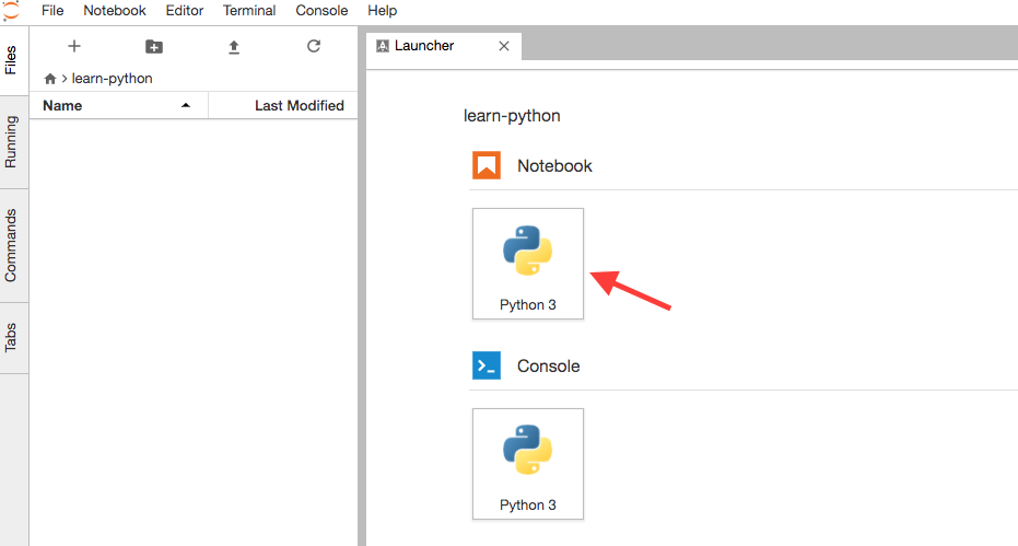
Let us start our first notebook by invoking Python 3 button under the Notebook symbol as shown below.

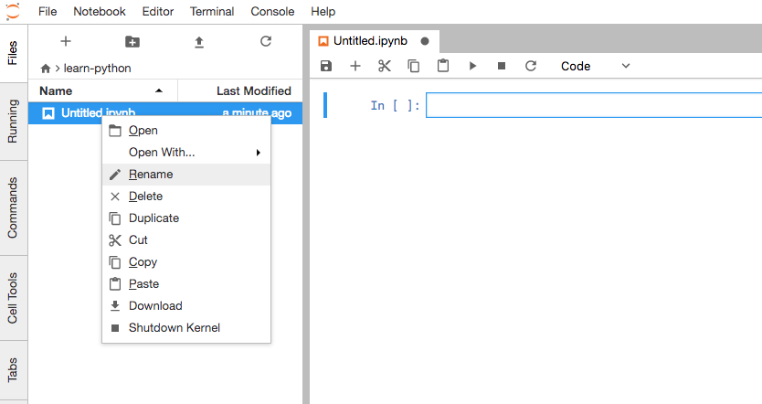
This will create a new file in learn-python folder with the name Untitled.ipynb by default. Change this name to firstConcept.ipynb by right clicking on the file and selecting rename as shown below.

What is .ipynb file
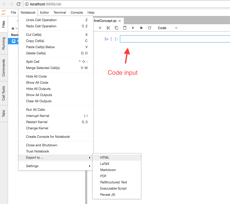
ipynb file extension is a notebook document used by Jupyter Notebook application. It contains all the information produced by Jupyter Notebook during a web application session which includes blocks of code, outputs from running the blocks of code, narratives, images, equations etc.. Contents are stored in plain JSON format. .ipynb files can be exported to other formats like HTML, PDF etc., as shown below. Once exported it is easy to share your work with others and also display it on the Web.

Notice the code input cell. Try inputting a few numbers and use it as a calculator to get started. For e.g.;
20 + 30
Press Ctrl+enter to run the calculation.
Then the output would be
50
You will notice a number within In[x] next to the code cell. x in this block contains a number which indicates the number of times that block is executed. If a block is still executing then you will see * in place of number. Once the execution is finished it increments to the next number.
You can add as many code input cells as you need in JupyterLab. In addition to code input cells, you can also add Markdown cells for narratives and Raw cells for code which is used for display only and not for evaluation. Both Markdown cells and Raw cells are not interpreted by Python Kernel.
Try adding a few more code cells and markdown cells for practice. Here are some of the most commonly used keyboard shortcuts you should be familiar with for Notebook, which help improve your efficiency: Point your mouse cursor on the left of the cell, as shown in the figure below to invoke keyboard shortcuts:

Keyboard shortcuts for notebook
| Short Cut | Result |
|---|---|
| a | Add a code cell above the current cell |
| b | Add a code cell below the current cell |
| dd | Delete the current cell |
| m | Covert the current cell to Markdown |
| y | Covert the current cell to Code cell |
| x | Cut selected cell |
| v | Paste cell below |
| l | Toggle line numbers |
| shift+tab | Helps to look up documentation on functions |
| ctrl+s | Save and check point |
| shift+enter | Execute the current code cell and jump to or create next code cell |
| ctrl+enter | Execute the current code cell |
| alt+enter | Execute the current code cell and create a new code cell below the current one |
Points to note
- You can expand or collapse a cell by toggling the cell marker on the left pane as shown below:

- To clear all outputs choose Notebook--> Clear All Outputs menu from toolbar
- There are more commands available in the same menu. Check them out. Help menu provides quick links to rich reference material of libraries and applications used for Data Science.
Few practice code cells you may add
You can use hash(#) for comments. Comments are not interpreted by the Python Kernel
# comments do not get executed.
width = 15
height = 10
area = width * height
print(area)
Out[x]:150
2 ** 3
Out[x]:8
You will notice that a print command was not required to see the output. Interpreter always outputs the last computed value and it also makes it available with a builtin variable _ which comes handy in case of interactive computing.
To time a code execution use %%time before you start the execution
%%time
2 ** 3
Out[x]: CPU times: user 2 µs, sys: 1e+03 ns, total: 3 µs Wall time: 5.01 µs
If you are familiar with working with Command prompt you can open command prompt right on notebook use %%bash
%%bash
pwd
/Users/home/python-tutorial/Exercises
How notebooks work
Notebook is a Web server. Web Server is nothing but a process which runs in an infinite loop and listens to user's connections from a browser. When it receives your request from the browser for a Web page, server returns a response HTML document. The server itself is not capable of running the Python program. Instead it opens a connection to Python Kernel and submits the code part of the Notebook to be processed by the Kernel. Once the Python Kernel processes the code, the Kernel returns the results back to the server. The server then returns the results to the browser. Browser displays it to the user.
Shutting down
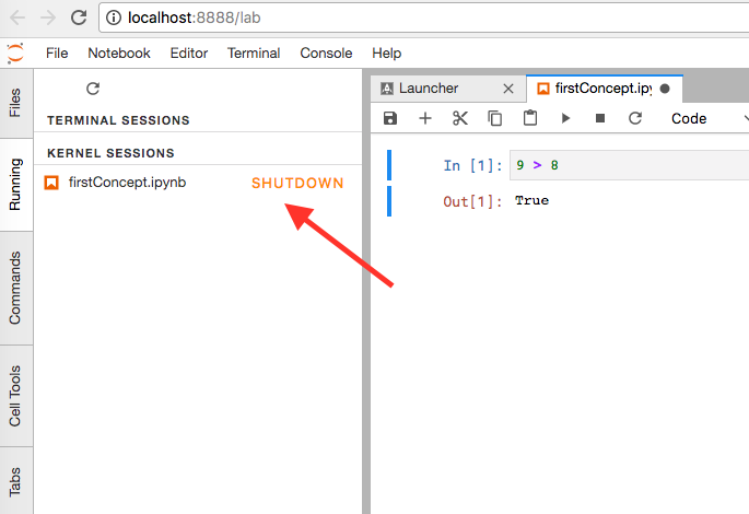
Individual notebook kernel can be shutdown by using the shutdown button in Running tab. See image below:

To stop the notebook server and the kernels of all notebooks, press Ctrl-C twice in the Terminal (Command prompt) console. Make sure your work is saved before shutting down!
References
While this book provides the necessary information to get started, you may refer to the official documentation as required on the website: http://jupyter-notebook.readthedocs.io/en/stable/notebook.html
Running Python programs from command line
You can also create a plain text file with just Python code in it and save it with .py extension. You can run this program on Python kernel by opening the Python interpreter from the Command prompt or Terminal by typing python or python3 and the name of the file.
Create a file called hello.py in any directory from any text editor of your choice and type in print("hello") and save it. Now from the Terminal or the Command prompt, navigate to the directory where you have the file saved by using cd. Once you are in the correct directory ensure that the file is present in that directory by running ls in Mac/Unix/Linux or dir in Windows. Then run python hello.py and you should see "hello" printed on the console.
